AftabRad Revit Add-in -> Export To Radiance -> Type of Sky/Analysis: Annual Sunlight Exposure by Rcontrib

This tutorial shows how to calculate the Annual Sunlight Exposure for selected calculation surface grids. This part of add-in helps Revit to communicate with Rcontrib in Radiance.

Moreover, since dynamic daylight analyses are usually based on the climate of the place, to calculate such metrics, we need to import the weather data file of the place too.

Anyway, as an example to do a Daylight Autonomy analysis for some of the rooms in the model, we should do the following steps.

1- Press calculationPointCreation button in the AftabRad Add-in

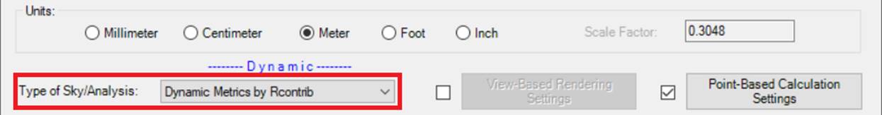
2- Select Dynamic Metrics by Rcontrib in the Type of Sky/Analysis

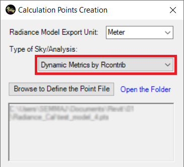
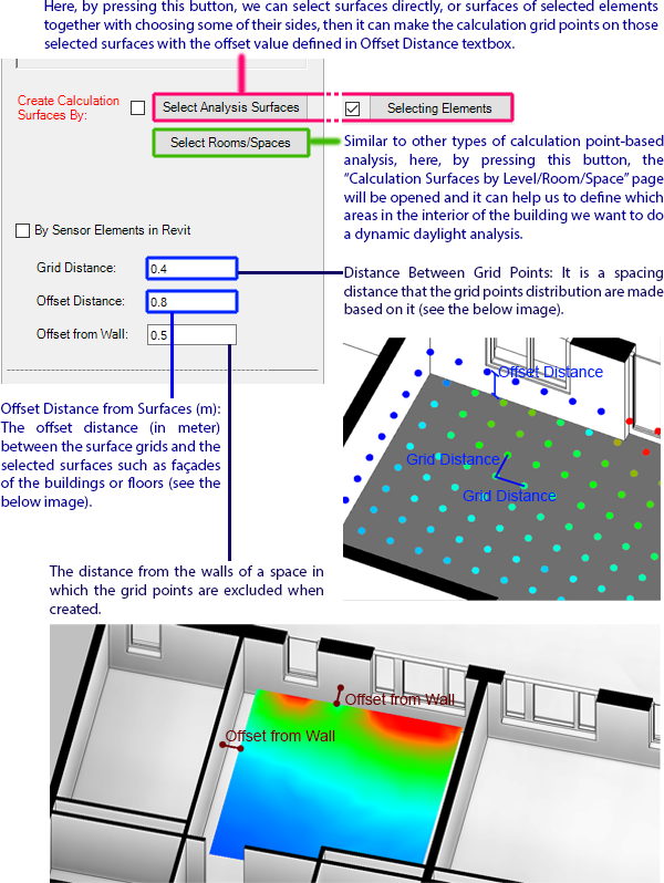
3- In the Calculation Point Creation page, we need to create calculation grids points by selecting some surfaces in the model, some elements together with choosing some of their surface normal directions,

or by choosing some of the rooms/spaces inside the building to do the analysis.

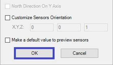
Now, we need to press the OK button in the Calculation Point Creation page.

4- Then we need to press ExportToRadiance button in the AftabRad Add-in

5- Check if the Dynamic Metrics by Rcontrib is chosen under the Type of Sky/Analysis. If not, please choose Dynamic Metrics by Rcontrib.as the Type of Sky/Analysis.

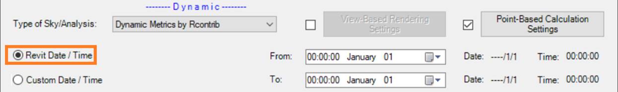
6- Any dynamic metrics is based on defining a period. So, in this add-in we can have two options to define the calculation period.

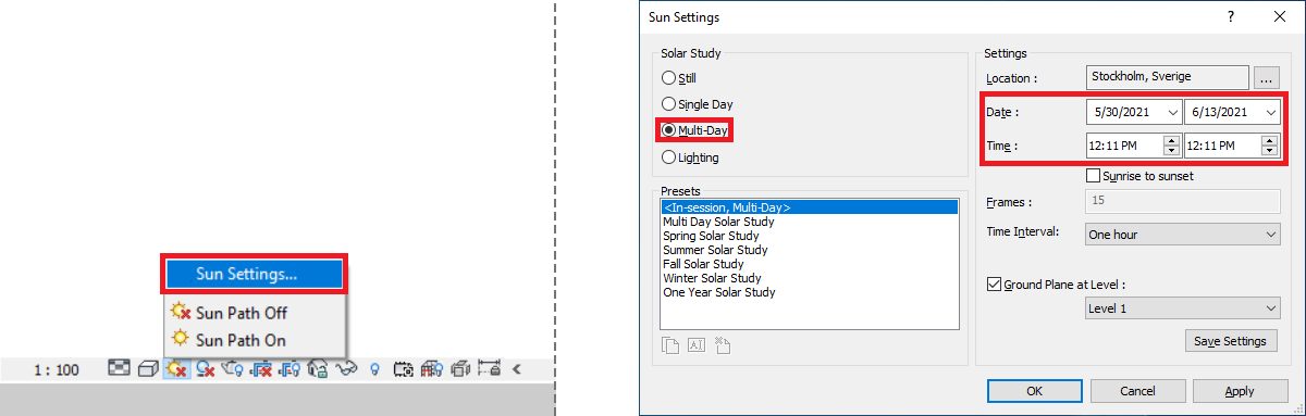
If we choose the Revit Date /Time radio button, the duration on which such an analysis is based on comes from the Sun Settings… in Revit.

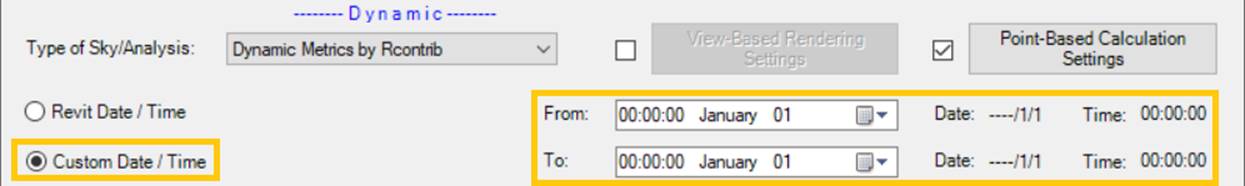
Otherwise, by choosing the the Custom Date /Time radio button, we can define the analysis period inside the Revit2Radiance page.

7- Since dynamic analyses are usually based on including typical weather conditions of the place, we need to import EPW (Energy Plus Weather Data File).

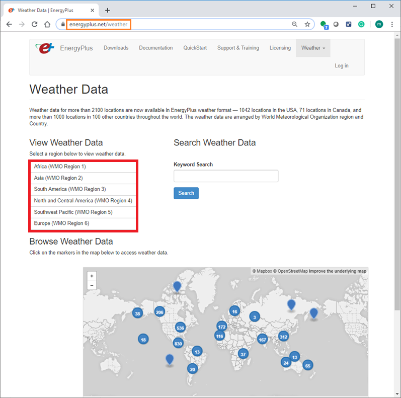
One of the most common way to find different EPW file for different cities in the world is to download the weather data file of around 2000 cities in the world from https://energyplus.net/weather website.

The other free option to find an appropriate EPW file for your project is to use this link: http://climate.onebuilding.org/

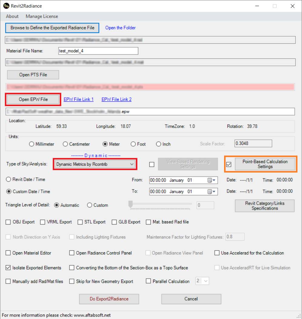
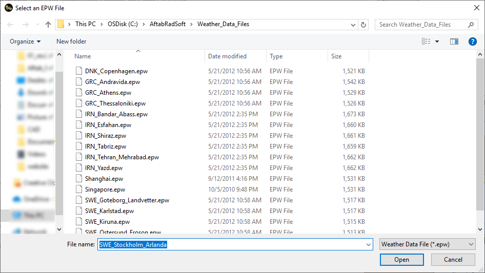
8- Press Open EPW File button and import an EPW file that is relevant to the location of your model.

9- Check the checkbox next to the Rtrace Settings button, and press the Do Export2Radiance button.

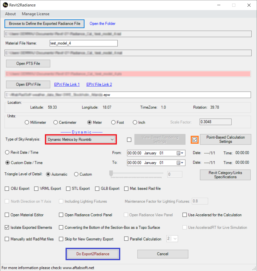
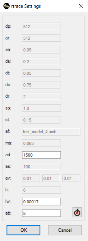
8- After pressing the Do Export2Radiance button, the simple rtrace Settings page will pops-up on the screen.

In this page, you can either confirm or modify the rtrace parameters that are used when measuring a daylight metric on any points in Radiance.

Between all the common rtrace parameters, three of them will be applied in the rcontrib based calculation. Between those three, the ab that shows the number of ambient bounces is the most important one.

However, the ambient divisions (ad) and limit the weight of each ray (lw) are the other parameters that can affect on the rcontrib calculations.

After finishing to change or confirm all the parameter values that are shown on this page, press the OK button to continue.

10- After pressing the OK button in the simple rtrace Settings page, a new page that is named Dynamic Inputs Form pops up on the screen.

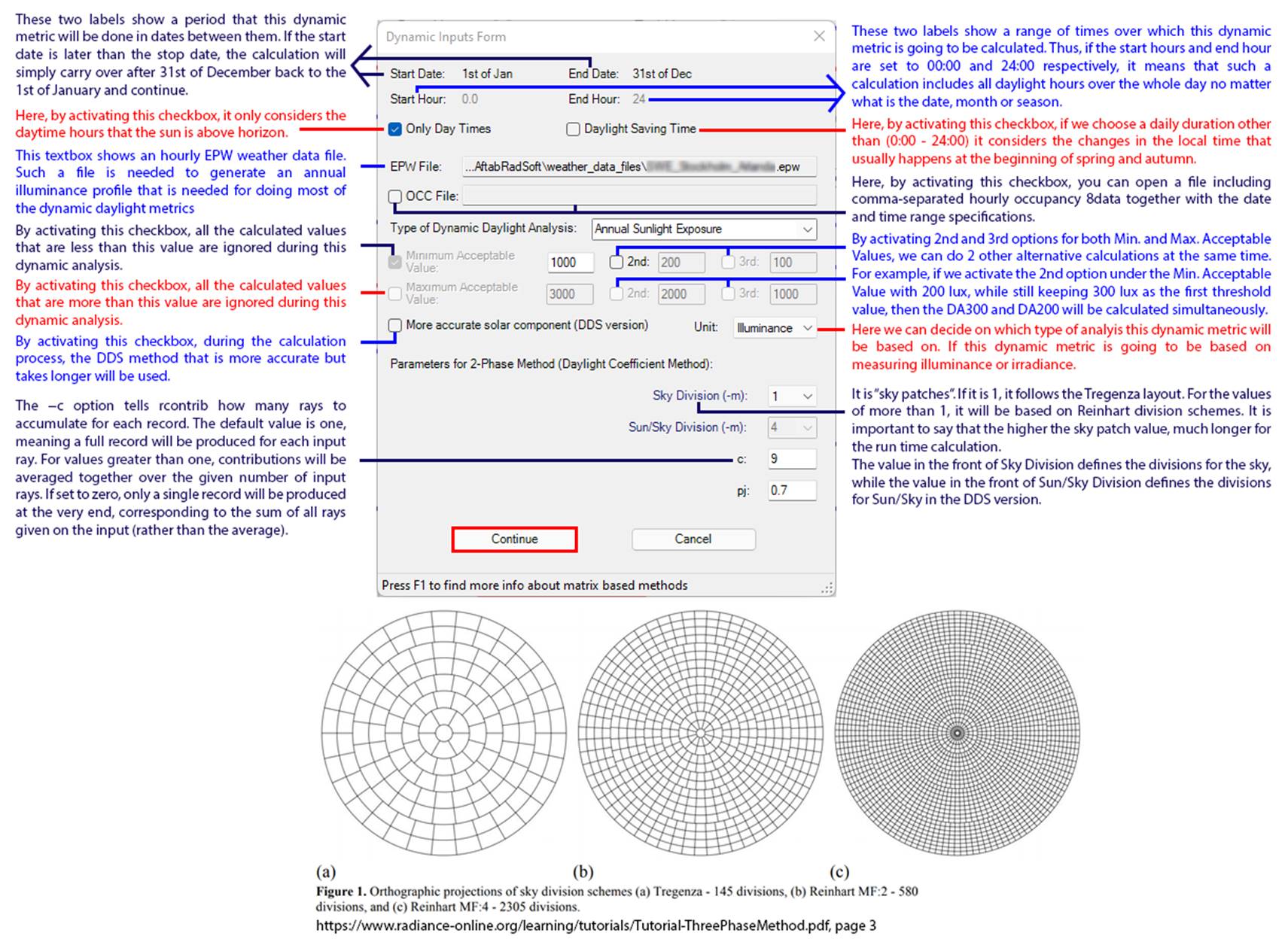
This page includes all the parameters that can help us to do a type dynamic daylight metric.

Here, in addition to showing the selected daily and yearly period, and the imported weather data file, it has other options like adding an occupancy file to define more precisely the working hours during a year, and Minimum and Maximum acceptable values.

In this page, we can also define if we want to do the illuminance or irradiance-based analysis. Here also we define the Sky Division or Sun/Sky Division that is needed by rcontrib to do such dynamic analysis.

The higher the Sky Division number, the more accurate results, but much longer the calculation time. To know more about all other parameters or options on this page, please take a look at the below image.

11- Moreover, in this page, under the Type of Analysis drop down list, you can find one of the following calculation types that are explained in the following:

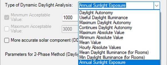
Daylight Autonomy:

It is a dynamic daylight performance measured at a certain point in the building. It is defined as the percentage of occupied hours per year when the minimum illuminance level can be maintained by daylight alone.

Useful Daylight Illuminance:

It is a dynamic daylight performance measured at a certain point in the building. It is defined as the percentage of occupied hours per year when daylight levels are 'useful' for the occupant, i.e. neither too dark (for example <100 lux) nor too bright (for example >3000 lux).

Maximum Daylight Autonomy:

It is a dynamic daylight performance measured at a certain point in the building. It is defined as the percentage of occupied hours per year when direct sunlight or exceedingly high daylight conditions are present.

It is based on measuring the number of hours when the daylight level is above the maximum illuminance level.

Continues Daylight Autonomy:

The continues daylight autonomy is a dynamic daylight performance measured at a certain point in the building. It is defined as the percentage of occupied hours per year when the minimum illuminance level can be maintained by daylight alone.

The difference between this metric and Daylight Autonomy is that in the Continues Daylight Autonomy even a partial contribution of daylight to illuminate a space is still beneficial.

Maximum Absolute Value:

By selecting this option, it measures the maximum absolute value of the selected period for each sensor.

Minimum Absolute Value:

By selecting this option, it measures the minimum absolute value of the selected period for each sensor.

Mean Value:

By selecting this option, it measures the average absolute value of the selected period for each sensor.

Hourly Absolute Values:

By selecting this option, it just creates separate calculation files for each hour in the selected period.

Annual Sunlight Exposure:

By selecting this option, it starts to do ASE (Annual Sunlight Exposure) calculation.

ASE is a metric that describes the potential for visual discomfort in interior work environments. It is defined as the number of hours per year that the selected point or area exceeds a specified direct sunlight illuminance level.

It is calculated BEFORE operable blinds and shades are deployed to block direct sunlight.

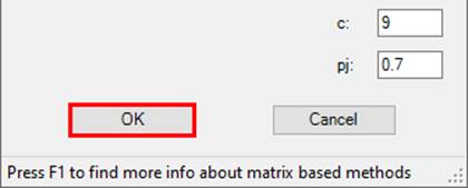
12- After doing all changes that are needed for our calculation on the Dynamic Inputs Form page, press the OK button.

13- As soon as pressing the OK button, firstly, a Dos command page like the one in the below will pop up on the screen

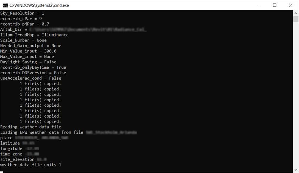
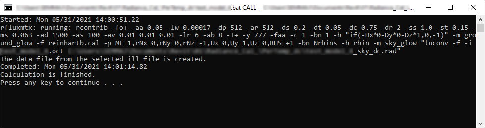
It will close in some seconds and then there will be another Dos command page (like the below image) that will pop up on the monitor.

As all the calculations that are related to the selected dynamic metric will be done in this step, it can take a while between some minutes to some hours depending on the complexity level of the model and number of calculation points.

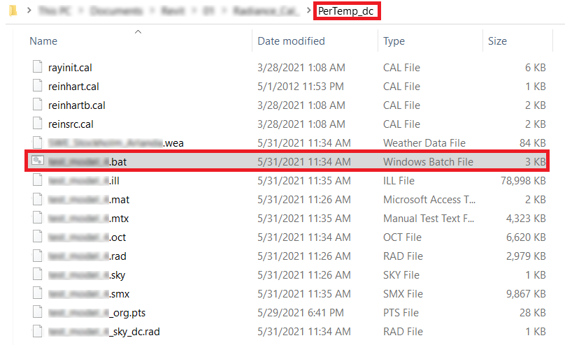
Here, it is worth saying that if you want to change some parameters or commands in the batch file, you should find the *.bat file under the PerTemp_dc folder that is created inside the calculation folder.

Then you need to open that batch file in programs like Notepad, Notepad++, and edit it and close it.

Finally, you need to re-run the batch file again by double click on that file.

14- Now, it is time to import the calculation data into Revit. Therefore, the next step is to press the importToRevit Button.

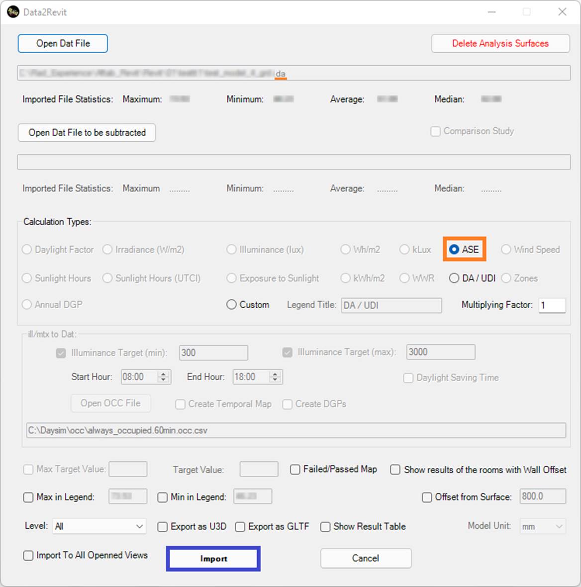
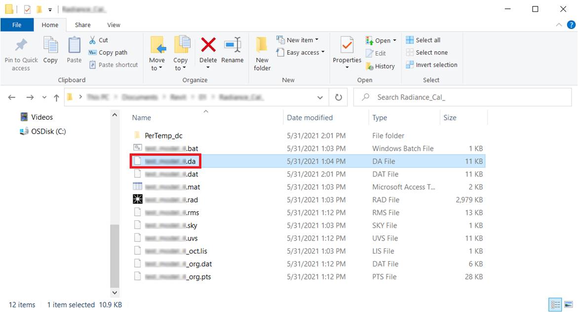
15- In the Data2Revit page, we need to press the Open Dat File button to open the right *.DA file.

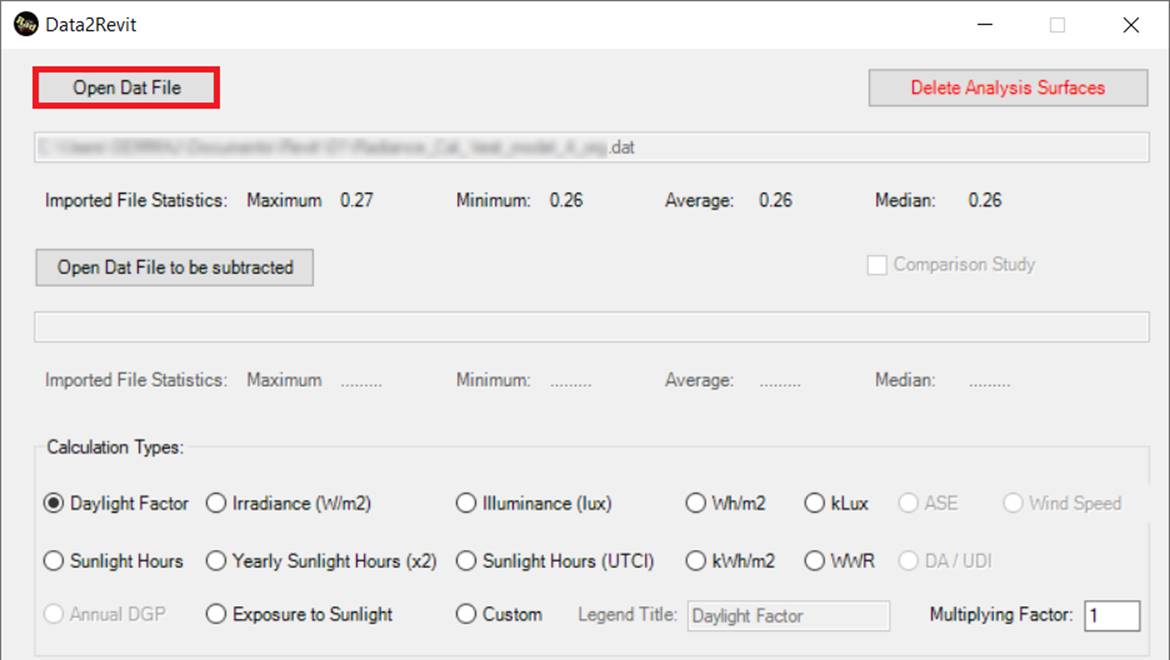
16- When pressing the Open Dat File button, the below page will be opened. Then we need to go where the *.da files are saved.

When choosing the right da file, press the Open button.

17- Select the DA/UDI under the Calculation Type and then press the Import button.